Table of Contents: |
Tree structures support various basic dynamic set operations including Search, Predecessor, Successor, Minimum, Maximum, Insert, and Delete in time proportional to the height of the tree. Ideally, a tree will be balanced and the height will be log n where n is the number of nodes in the tree. To ensure that the height of the tree is as small as possible and therefore provide the best running time, a balanced tree structure like a red-black tree, AVL tree, or b-tree must be used.
When working with large sets of data, it is often not possible or desirable to maintain the entire structure in primary storage (RAM). Instead, a relatively small portion of the data structure is maintained in primary storage, and additional data is read from secondary storage as needed. Unfortunately, a magnetic disk, the most common form of secondary storage, is significantly slower than random access memory (RAM). In fact, the system often spends more time retrieving data than actually processing data.
B-trees are balanced trees that are optimized for situations when part or all of the tree must be maintained in secondary storage such as a magnetic disk. Since disk accesses are expensive (time consuming) operations, a b-tree tries to minimize the number of disk accesses. For example, a b-tree with a height of 2 and a branching factor of 1001 can store over one billion keys but requires at most two disk accesses to search for any node (Cormen 384).
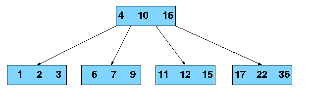
Unlike a binary-tree, each node of a b-tree may have a variable number of keys and children. The keys are stored in non-decreasing order. Each key has an associated child that is the root of a subtree containing all nodes with keys less than or equal to the key but greater than the preceeding key. A node also has an additional rightmost child that is the root for a subtree containing all keys greater than any keys in the node.
A b-tree has a minumum number of allowable children for each node known as the minimization factor. If t is this minimization factor, every node must have at least t - 1 keys. Under certain circumstances, the root node is allowed to violate this property by having fewer than t - 1 keys. Every node may have at most 2t - 1 keys or, equivalently, 2t children.
Since each node tends to have a large branching factor (a large number of children), it is typically neccessary to traverse relatively few nodes before locating the desired key. If access to each node requires a disk access, then a b-tree will minimize the number of disk accesses required. The minimzation factor is usually chosen so that the total size of each node corresponds to a multiple of the block size of the underlying storage device. This choice simplifies and optimizes disk access. Consequently, a b-tree is an ideal data structure for situations where all data cannot reside in primary storage and accesses to secondary storage are comparatively expensive (or time consuming).
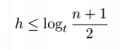
For n greater than or equal to one, the height of an n-key b-tree T of height h with a minimum degree t greater than or equal to 2,
The worst case height is O(log n). Since the "branchiness" of a b-tree can be large compared to many other balanced tree structures, the base of the logarithm tends to be large; therefore, the number of nodes visited during a search tends to be smaller than required by other tree structures. Although this does not affect the asymptotic worst case height, b-trees tend to have smaller heights than other trees with the same asymptotic height.
The algorithms for the search, create, and insert operations are shown below. Note that these algorithms are single pass; in other words, they do not traverse back up the tree. Since b-trees strive to minimize disk accesses and the nodes are usually stored on disk, this single-pass approach will reduce the number of node visits and thus the number of disk accesses. Simpler double-pass approaches that move back up the tree to fix violations are possible.
Since all nodes are assumed to be stored in secondary storage (disk) rather than primary storage (memory), all references to a given node be be preceeded by a read operation denoted by Disk-Read. Similarly, once a node is modified and it is no longer needed, it must be written out to secondary storage with a write operation denoted by Disk-Write. The algorithms below assume that all nodes referenced in parameters have already had a corresponding Disk-Read operation. New nodes are created and assigned storage with the Allocate-Node call. The implementation details of the Disk-Read, Disk-Write, and Allocate-Node functions are operating system and implementation dependent.
i <- 1
while i <= n[x] and k > keyi[x]
     do i <- i + 1
if i <= n[x] and k = keyi[x]
     then return (x, i)
if leaf[x]
     then return NIL
     else Disk-Read(ci[x])
          return B-Tree-Search(ci[x], k)
The search operation on a b-tree is analogous to a search on a binary tree. Instead of choosing between a left and a right child as in a binary tree, a b-tree search must make an n-way choice. The correct child is chosen by performing a linear search of the values in the node. After finding the value greater than or equal to the desired value, the child pointer to the immediate left of that value is followed. If all values are less than the desired value, the rightmost child pointer is followed. Of course, the search can be terminated as soon as the desired node is found. Since the running time of the search operation depends upon the height of the tree, B-Tree-Search is O(logt n).
x <- Allocate-Node()
leaf[x] <- TRUE
n[x] <- 0
Disk-Write(x)
root[T] <- x
The B-Tree-Create operation creates an empty b-tree by allocating a new root node that has no keys and is a leaf node. Only the root node is permitted to have these properties; all other nodes must meet the criteria outlined previously. The B-Tree-Create operation runs in time O(1).
z <- Allocate-Node()
leaf[z] <- leaf[y]
n[z] <- t - 1
for j <- 1 to t - 1
     do keyj[z] <- keyj+t[y]
if not leaf[y]
     then for j <- 1 to t
          do cj[z] <- cj+t[y]
n[y] <- t - 1
for j <- n[x] + 1 downto i + 1
     do cj+1[x] <- cj[x]
ci+1 <- z
for j <- n[x] downto i
     do keyj+1[x] <- keyj[x]
keyi[x] <- keyt[y]
n[x] <- n[x] + 1
Disk-Write(y)
Disk-Write(z)
Disk-Write(x)
If is node becomes "too full," it is necessary to perform a split operation. The split operation moves the median key of node x into its parent y where x is the ith child of y. A new node, z, is allocated, and all keys in x right of the median key are moved to z. The keys left of the median key remain in the original node x. The new node, z, becomes the child immediately to the right of the median key that was moved to the parent y, and the original node, x, becomes the child immediately to the left of the median key that was moved into the parent y.
The split operation transforms a full node with 2t - 1 keys into two nodes with t - 1 keys each. Note that one key is moved into the parent node. The B-Tree-Split-Child algorithm will run in time O(t) where t is constant.
r <- root[T]
if n[r] = 2t - 1
     then s <- Allocate-Node()
          root[T] <- s
	  leaf[s] <- FALSE
	  n[s] <- 0
	  c1 <- r
	  B-Tree-Split-Child(s, 1, r)
	  B-Tree-Insert-Nonfull(s, k)
     else B-Tree-Insert-Nonfull(r, k)
i <- n[x]
if leaf[x]
     then while i >= 1 and k < keyi[x]
            do keyi+1[x] <- keyi[x]
	       i <- i - 1
          keyi+1[x] <- k
	  n[x] <- n[x] + 1
	  Disk-Write(x)
     else while i >= and k < keyi[x]
            do i <- i - 1
	  i <- i + 1
	  Disk-Read(ci[x])
	  if n[ci[x]] = 2t - 1
	       then B-Tree-Split-Child(x, i, ci[x])
	            if k > keyi[x]
		         then i <- i + 1
          B-Tree-Insert-Nonfull(ci[x], k)
To perform an insertion on a b-tree, the appropriate node for the key must be located using an algorithm similiar to B-Tree-Search. Next, the key must be inserted into the node. If the node is not full prior to the insertion, no special action is required; however, if the node is full, the node must be split to make room for the new key. Since splitting the node results in moving one key to the parent node, the parent node must not be full or another split operation is required. This process may repeat all the way up to the root and may require splitting the root node. This approach requires two passes. The first pass locates the node where the key should be inserted; the second pass performs any required splits on the ancestor nodes.
Since each access to a node may correspond to a costly disk access, it is desirable to avoid the second pass by ensuring that the parent node is never full. To accomplish this, the presented algorithm splits any full nodes encountered while descending the tree. Although this approach may result in unecessary split operations, it guarantees that the parent never needs to be split and eliminates the need for a second pass up the tree. Since a split runs in linear time, it has little effect on the O(t logt n) running time of B-Tree-Insert.
Splitting the root node is handled as a special case since a new root must be created to contain the median key of the old root. Observe that a b-tree will grow from the top.
Deletion of a key from a b-tree is possible; however, special care must be taken to ensure that the properties of a b-tree are maintained. Several cases must be considered. If the deletion reduces the number of keys in a node below the minimum degree of the tree, this violation must be corrected by combining several nodes and possibly reducing the height of the tree. If the key has children, the children must be rearranged. For a detailed discussion of deleting from a b-tree, refer to Section 19.3, pages 395-397, of Cormen, Leiserson, and Rivest or to another reference listed below.

A database is a collection of data organized in a fashion that facilitates updating, retrieving, and managing the data. The data can consist of anything, including, but not limited to names, addresses, pictures, and numbers. Databases are commonplace and are used everyday. For example, an airline reservation system might maintain a database of available flights, customers, and tickets issued. A teacher might maintain a database of student names and grades.
Because computers excel at quickly and accurately manipulating, storing, and retrieving data, databases are often maintained electronically using a database management system. Database management systems are essential components of many everyday business operations. Database products like Microsoft SQL Server, Sybase Adaptive Server, IBM DB2, and Oracle serve as a foundation for accounting systems, inventory systems, medical recordkeeping sytems, airline reservation systems, and countless other important aspects of modern businesses.
It is not uncommon for a database to contain millions of records requiring many gigabytes of storage. For examples, TELSTRA, an Australian telecommunications company, maintains a customer billing database with 51 billion rows (yes, billion) and 4.2 terabytes of data. In order for a database to be useful and usable, it must support the desired operations, such as retrieval and storage, quickly. Because databases cannot typically be maintained entirely in memory, b-trees are often used to index the data and to provide fast access. For example, searching an unindexed and unsorted database containing n key values will have a worst case running time of O(n); if the same data is indexed with a b-tree, the same search operation will run in O(log n). To perform a search for a single key on a set of one million keys (1,000,000), a linear search will require at most 1,000,000 comparisons. If the same data is indexed with a b-tree of minimum degree 10, 114 comparisons will be required in the worst case. Clearly, indexing large amounts of data can significantly improve search performance. Although other balanced tree structures can be used, a b-tree also optimizes costly disk accesses that are of concern when dealing with large data sets.
Databases typically run in multiuser environments where many users can concurrently perform operations on the database. Unfortunately, this common scenario introduces complications. For example, imagine a database storing bank account balances. Now assume that someone attempts to withdraw $40 from an account containing $60. First, the current balance is checked to ensure sufficent funds. After funds are disbursed, the balance of the account is reduced. This approach works flawlessly until concurrent transactions are considered. Suppose that another person simultaneously attempts to withdraw $30 from the same account. At the same time the account balance is checked by the first person, the account balance is also retrieved for the second person. Since neither person is requesting more funds than are currently available, both requests are satisfied for a total of $70. After the first person's transaction, $20 should remain ($60 - $40), so the new balance is recorded as $20. Next, the account balance after the second person's transaction, $30 ($60 - $30), is recorded overwriting the $20 balance. Unfortunately, $70 have been disbursed, but the account balance has only been decreased by $30. Clearly, this behavior is undesirable, and special precautions must be taken.
A b-tree suffers from similar problems in a multiuser environment. If two or more processes are manipulating the same tree, it is possible for the tree to become corrupt and result in data loss or errors.
The simplest solution is to serialize access to the data structure. In other words, if another process is using the tree, all other processes must wait. Although this is feasible in many cases, it can place an unecessary and costly limit on performance because many operations actually can be performed concurrently without risk. Locking, introduced by Gray and refined by many others, provides a mechanism for controlling concurrent operations on data structures in order to prevent undesirable side effects and to ensure consistency. For a detailed discussion of this and other concurrency control mechanisms, please refer to the references below.